
Cardinality estimation and performance are linked. The optimizer guesses how many rows each step returns, and that guess picks the plan. I tested one query under both estimators on SQL Server 2025 to see what a better guess is worth.

What Cardinality Means
Cardinality is the number of rows an operator returns. Before SQL Server runs a query, it estimates that number for every step, using statistics. Those estimates decide three things: seek or scan, which join to use, and how much memory to ask for. That is why cardinality estimation and performance cannot be separated. A wrong estimate wastes reads, CPU and memory in one query.
The code that makes these estimates is the cardinality estimator. For years it never changed. SQL Server 2014 replaced it with a new design that turns on at compatibility level 120 and higher. The old design is now called the legacy estimator. My test database is at level 170, so every query uses the new one unless I ask otherwise.
Here is my sixty second video on the idea.
A Table Where Two Columns Move Together
The two estimators differ most when a query filters on two columns at once. The legacy one assumes the columns are unrelated and multiplies the two selectivities. The new one assumes some overlap, so it softens the second filter and returns a larger number. City and state are a good example of columns that move together.
The test table holds 200,000 customers. Every Portland customer lives in Oregon, so the two filters overlap fully. The Tier column is in neither index, and that matters later.
IF DB_ID(N'SqlCardinalityDemo') IS NULL CREATE DATABASE SqlCardinalityDemo;
GO
USE SqlCardinalityDemo;
GO
DROP TABLE IF EXISTS dbo.Customers;
CREATE TABLE dbo.Customers
(
    CustomerID int IDENTITY(1,1) PRIMARY KEY,
    City varchar(30) NOT NULL,
    State char(2) NOT NULL,
    Tier char(1) NOT NULL DEFAULT 'A'
);
INSERT INTO dbo.Customers (City, State)
SELECT p.City, p.State
FROM GENERATE_SERIES(1, 200000) AS s
JOIN (VALUES (0, 'Portland', 'OR'), (1, 'Eugene', 'OR'), (2, 'Salem', 'OR'), (3, 'Seattle', 'WA'),
             (4, 'Tacoma', 'WA'), (5, 'Spokane', 'WA'), (6, 'Boise', 'ID'), (7, 'Austin', 'TX'),
             (8, 'Dallas', 'TX'), (9, 'Houston', 'TX'), (10, 'Denver', 'CO'), (11, 'Boulder', 'CO'),
             (12, 'Phoenix', 'AZ'), (13, 'Tucson', 'AZ'), (14, 'Reno', 'NV'), (15, 'Fresno', 'CA'),
             (16, 'Oakland', 'CA'), (17, 'Chicago', 'IL'), (18, 'Peoria', 'IL'), (19, 'Madison', 'WI'),
             (20, 'Boston', 'MA'), (21, 'Newton', 'MA'), (22, 'Albany', 'NY'), (23, 'Buffalo', 'NY'),
             (24, 'Miami', 'FL')) AS p (Slot, City, State) ON p.Slot = s.value % 25;
CREATE INDEX IX_Customers_City ON dbo.Customers (City);
CREATE INDEX IX_Customers_State ON dbo.Customers (State);
Each city holds 8,000 rows. Oregon has three cities, so it holds 24,000. The query below confirms the overlap.
SELECT SUM(CASE WHEN City = 'Portland' THEN 1 ELSE 0 END) AS Portland,
       SUM(CASE WHEN State = 'OR' THEN 1 ELSE 0 END) AS Oregon,
       SUM(CASE WHEN City = 'Portland' AND State = 'OR' THEN 1 ELSE 0 END) AS Both
FROM dbo.Customers;| Portland | Oregon | Both |
|---|---|---|
| 8,000 | 24,000 | 8,000 |
One Query, Two Estimates
Now run one query twice. The hint on the second copy forces the legacy estimator for that statement only. Turn on Include Actual Execution Plan (Ctrl+M) first. Then compare the estimated and actual rows on the scan or the seeks.
SET STATISTICS IO ON;
SELECT CustomerID, City, State, Tier FROM dbo.Customers WHERE City = 'Portland' AND State = 'OR';
SELECT CustomerID, City, State, Tier FROM dbo.Customers WHERE City = 'Portland' AND State = 'OR'
OPTION (USE HINT('FORCE_LEGACY_CARDINALITY_ESTIMATION'));| Estimator | Estimated rows | Actual rows | Plan | Logical reads |
|---|---|---|---|---|
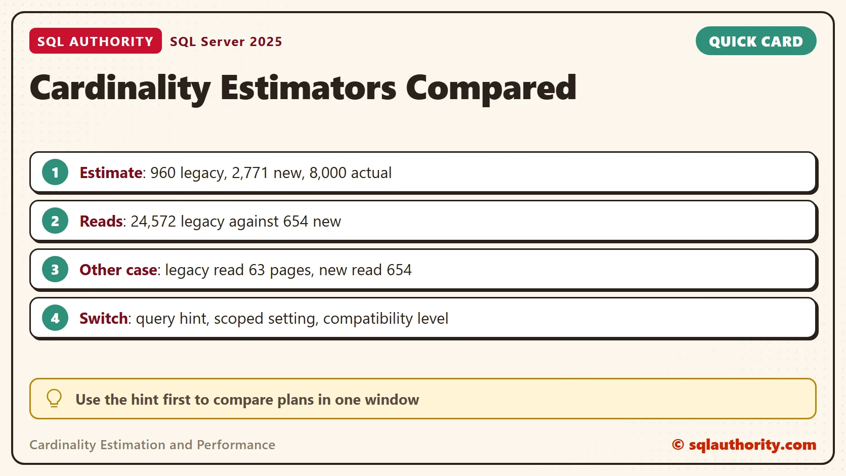
| New (default) | 2,771 | 8,000 | Clustered index scan | 654 |
| Legacy | 960 | 8,000 | Two index seeks, a merge join, key lookups | 24,572 |
The legacy math is simple. Portland is 4 percent of the table and Oregon is 12 percent. Four percent of 12 percent of 200,000 rows is 960.
The new estimator keeps the most selective filter at full strength. It then multiplies by the square root of the next one. Four percent times the square root of 12 percent is about 1.4 percent, and that is 2,771 rows. Both estimates are too low, because the real answer is 8,000. The legacy guess is off by a factor of eight, and the new guess by a factor of three.
That difference changed the plan. With 960 rows, looking up Tier one row at a time looked cheap. With 2,771 rows, a single scan looked cheaper. The scan was the right call: it read 654 pages, while the lookups read 24,572, about 38 times more.
You can see which estimator ran. Click the SELECT operator at the top of the plan and open its Properties window. The field Cardinality Estimation Model Version shows 170 for the new estimator and 70 for the legacy one. In my run, the plain query showed 170 and the hinted query showed 70.
When the New Guess Costs You
No estimator wins every query. A guess only matters when it crosses the point where one plan becomes cheaper than the other. Now ask for Portland in Washington. No such customers exist, so the real answer is zero rows.
SELECT CustomerID, City, State, Tier FROM dbo.Customers WHERE City = 'Portland' AND State = 'WA';
SELECT CustomerID, City, State, Tier FROM dbo.Customers WHERE City = 'Portland' AND State = 'WA'
OPTION (USE HINT('FORCE_LEGACY_CARDINALITY_ESTIMATION'));
The estimates did not move: 2,771 for the new estimator and 960 for the legacy one. This time the legacy plan won. It merged the two indexes, found nothing, and read 63 pages. The new plan scanned the whole table and read 654, about ten times more.
A query with one filter gets the same estimate under both. Portland alone is estimated at 8,000 rows by each estimator, because the statistics on City say so. Both pick the same scan with 654 reads, so logical reads do not change.
You could say a 200,000 row table is too small to matter, and both plans finish in milliseconds. Fair point. The ratio comes from the plan shape, though, so a larger table keeps the ratio and multiplies the cost.
Switch With the Smallest Change
Three switches exist, from narrow to wide. The query hint changes one statement. The database scoped configuration changes one database. Setting the compatibility level below 120 changes everything and also gives up newer features.
ALTER DATABASE SCOPED CONFIGURATION SET LEGACY_CARDINALITY_ESTIMATION = ON;
ALTER DATABASE SCOPED CONFIGURATION SET LEGACY_CARDINALITY_ESTIMATION = OFF;
Use the hint first. It lets you compare the two plans in one window and leaves every other query alone. The database setting is a stopgap for an upgrade where many queries slowed at once. Remove it as soon as you have fixed the worst queries.
A Simple Rule
Tune cardinality estimation and performance after an upgrade by reading the estimated and actual rows first. A big gap points to a data problem the estimator cannot see. Here, the fix is a statistics object that covers both columns.
CREATE STATISTICS ST_Customers_City_State ON dbo.Customers (City, State) WITH FULLSCAN;
With that object in place, both estimators guessed 8,000 for the Oregon query, and both chose the 654 read scan. Fix the data the optimizer sees, then keep the new estimator for the rest of your workload. Test on a copy with production-sized data. Estimates follow the shape of the data, not the size of the server. Newer features, such as cardinality estimation feedback in SQL Server 2022, build on it. In short, cardinality estimation and performance both depend on what the optimizer can see.
When you finish testing, remove the example database.
USE master;
GO
ALTER DATABASE SqlCardinalityDemo SET SINGLE_USER WITH ROLLBACK IMMEDIATE;
DROP DATABASE SqlCardinalityDemo;
A cardinality estimate is not a fact, it is a bet that the whole plan is built on.
Published by Pinal Dave on SQLAuthority. More of my work at pinaldave.com.
Discover more from SQL Authority with Pinal Dave
Subscribe to get the latest posts sent to your email.




2 Comments. Leave new
Hi I tried this feature on SQL Server 2017 but for me there is no change in logical reads. Every time its same. I tried the code as in your example.
Table ‘Customers’. Scan count 1, logical reads 104, physical reads 0, read-ahead reads 0, lob logical reads 0, lob physical reads 0, lob read-ahead reads 0.
Table ‘Customers’. Scan count 1, logical reads 104, physical reads 0, read-ahead reads 0, lob logical reads 0, lob physical reads 0, lob read-ahead reads 0.
Not every query would benefit from new CE.