Value Histograms: Counting Rows per Range Bucket in T-SQL

Value histograms turn a long column of numbers into a short list of ranges and how many rows fall in each. One GROUP BY gets you started. Three small traps decide whether the answer is true.

Twenty orders and one expression

Say a manager asks, “How are our order amounts spread out?” A list of twenty amounts does not answer that. Buckets of 100 do. The setup below creates twenty orders. Run it first.

DROP TABLE IF EXISTS #Sales;
CREATE TABLE #Sales (SaleId int PRIMARY KEY, Amount decimal(10,2) NOT NULL);
INSERT #Sales VALUES
    (1, 12.50), (2, 45.00), (3, 99.99), (4, 100.00), (5, 135.25),
    (6, 180.00), (7, 199.99), (8, 200.00), (9, 215.40), (10, 240.00),
    (11, 275.10), (12, 505.75), (13, 520.00), (14, 560.20), (15, 610.00),
    (16, 95.00), (17, 150.00), (18, 130.00), (19, 750.00), (20, 20.00);

The bucket start is Amount divided by the bucket width, rounded down, then multiplied back. That one expression is the heart of every histogram you will write.

SELECT CAST(FLOOR(Amount / 100) AS int) * 100 AS BucketStart,
       COUNT(*) AS Orders
FROM #Sales
GROUP BY CAST(FLOOR(Amount / 100) AS int) * 100
ORDER BY BucketStart;

Six rows come back: 0, 100, 200, 500, 600 and 700. Look closely. There is no 300 and no 400. That is trap number one.

Empty buckets vanish unless you ask for them

GROUP BY can only report groups that have rows. A bucket with zero orders has no rows, so it silently disappears. On a chart, the gap between 200 and 500 would look like the bars simply touch each other. Readers draw the wrong conclusion.

The fix is to list every bucket yourself and LEFT JOIN the data to it. Here I also show the mistake that goes with it. COUNT(*) counts the join row itself, so an empty bucket reports 1 instead of 0.

SELECT b.BucketStart,
       COUNT(*) AS WrongCount,
       COUNT(s.SaleId) AS Orders
FROM (VALUES (0), (100), (200), (300), (400), (500), (600), (700)) AS b(BucketStart)
LEFT JOIN #Sales AS s
    ON s.Amount >= b.BucketStart
   AND s.Amount < b.BucketStart + 100
GROUP BY b.BucketStart
ORDER BY b.BucketStart;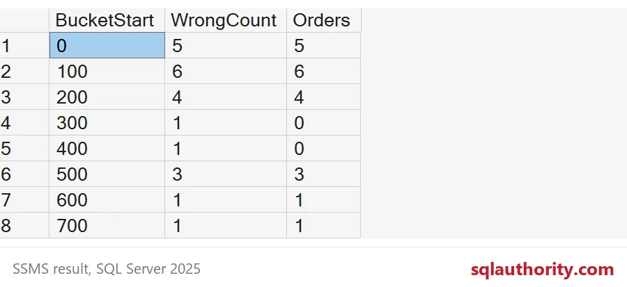

Now eight rows appear, with 300 and 400 showing 0 under Orders. WrongCount shows 1 for both. Counting a column from the right-hand table, one that is never NULL when a match exists, is the habit that saves you.

When the buckets are not the same width

Real reports rarely use equal widths. Small, medium, large and huge orders are more useful to a manager than eight even slices. For that, put the ranges in a small table. Each range has a lower bound that is included and an upper bound that is not.

DROP TABLE IF EXISTS #Ranges;
CREATE TABLE #Ranges (RangeNo int PRIMARY KEY, Label varchar(20) NOT NULL,
                      LowerBound decimal(10,2) NOT NULL, UpperBound decimal(10,2) NOT NULL);
INSERT #Ranges VALUES
    (1, 'Under 50', 0, 50), (2, '50 to 199', 50, 200),
    (3, '200 to 499', 200, 500), (4, '500 and up', 500, 1000000);

SELECT r.Label, COUNT(s.SaleId) AS Orders
FROM #Ranges AS r
LEFT JOIN #Sales AS s
    ON s.Amount >= r.LowerBound
   AND s.Amount < r.UpperBound
GROUP BY r.RangeNo, r.Label
ORDER BY r.RangeNo;

The counts are 3, 8, 4 and 5, adding up to the twenty orders. A range table also lets a business user change the cut points without touching the query.

The BETWEEN trap

Here is trap number three, and I see it in code reviews every month. BETWEEN includes both ends. Two neighboring buckets written with BETWEEN both claim the value that sits on the border. Order 4 is exactly 100.00, and order 8 is exactly 200.00.

SELECT
    SUM(CASE WHEN Amount BETWEEN 0 AND 100 THEN 1 ELSE 0 END)
  + SUM(CASE WHEN Amount BETWEEN 100 AND 200 THEN 1 ELSE 0 END) AS BetweenTotal,
    SUM(CASE WHEN Amount >= 0 AND Amount < 100 THEN 1 ELSE 0 END)
  + SUM(CASE WHEN Amount >= 100 AND Amount < 200 THEN 1 ELSE 0 END) AS HalfOpenTotal
FROM #Sales;

The real number of orders below 200 is 11. The half-open version says 11. The BETWEEN version says 13. The 100.00 order was counted twice, and the 200.00 order was pulled into a bucket where it does not belong. Write every bucket as “greater than or equal to the start, less than the next start” and the borders behave.

Draw it right in the result grid

You do not need a charting tool to see the shape. REPLICATE can draw a bar from the count. It works well for the equal-width buckets only. With uneven ranges, a wide bucket holds more rows just by being wide, so compare those by count per unit of width.

SELECT b.BucketStart,
       COUNT(s.SaleId) AS Orders,
       REPLICATE('#', COUNT(s.SaleId)) AS Bar
FROM (VALUES (0), (100), (200), (300), (400), (500), (600), (700)) AS b(BucketStart)
LEFT JOIN #Sales AS s
    ON s.Amount >= b.BucketStart
   AND s.Amount < b.BucketStart + 100
GROUP BY b.BucketStart
ORDER BY b.BucketStart;

DROP TABLE IF EXISTS #Ranges;
DROP TABLE IF EXISTS #Sales;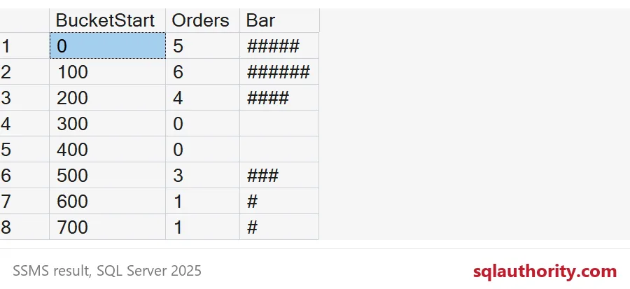

The bars make the two empty buckets obvious, and the lonely order at 750 stands out. Next time someone asks how the numbers are spread, you can show the shape before they finish the sentence.

A histogram is not a count, it is a shape.

Published by Pinal Dave on SQLAuthority. More of my work at pinaldave.com.