I let AI recommend SQL Server indexes across a week of queries, measured every number before and after, and the result was not the one I expected to write about.

I expected a comedy. I have read enough confident nonsense from chatbots about SQL Server to assume I would end up with a post full of terrible indexes and easy jokes.
That is not what happened, and the actual answer is more useful.
AI never connected to SQL Server or executed anything. I gave a general-purpose chat model one query at a time, manually reviewed its suggestions, and applied the candidates in a disposable lab database. This is a case study of that copy-and-paste workflow, not a benchmark of every model and not autonomous index management.
The Rules I Set Myself
One rule mattered more than the rest. AI only saw what a typical copy-and-paste chat receives. The table definitions and the query text. No execution plans, no statistics, no wait stats, no data distribution, and no list of the indexes that already existed.
That is not me being unfair to it. That is the situation almost every person is in when they paste a slow query into a chat window and ask what index they need.
Two honest notes about method. I structured the experiment as a Monday-to-Friday week of queries, but ran it in one sitting. I also started each query without telling the model what came before. Model answers can change over time, so treat this as one observed run, not a permanent score. Every reported result is measured rather than remembered.
Monday. The Blank Slate
A small e-commerce shape. Nothing exotic.
| Table | Rows |
|---|---|
| Customers | 50,000 |
| Products | 2,000 |
| Orders | 300,000 |
| OrderItems | 900,000 |
Every table had a clustered primary key and nothing else. No nonclustered indexes anywhere. The data is generated deterministically. The script at the end reproduces the write-cost test rather than the whole six-query benchmark.
Six queries, each run six times, whole set repeated three times, then averaged. Logical reads are stable to the page. Durations wander, so I never trusted a single run.
| Query | Logical reads | Duration |
|---|---|---|
| Q1 orders for a customer | 3,965 | 26.6 ms |
| Q2 pending orders | 3,965 | 37.0 ms |
| Q3 items for a product | 3,573 | 59.7 ms |
| Q4 customer by email | 864 | 5.9 ms |
| Q5 top products | 7,538 | 119.8 ms |
| Q6 country and status | 3,965 | 41.1 ms |
| Total | 23,870 | 290.1 ms |
With only clustered primary keys available, each query relied on at least one clustered index scan. SQL Server was reading far more pages than the selective queries needed.
Tuesday. The Four Easy Ones
I handed over the first four queries, one at a time. Here is the first, and what came back.
SELECT COUNT(*), SUM(TotalDue)
FROM dbo.Orders
WHERE CustomerID = 24680
  AND OrderDate >= '2026-01-01' AND OrderDate < '2026-08-01';

CREATE NONCLUSTERED INDEX IX_Orders_CustomerID_OrderDate
    ON dbo.Orders (CustomerID, OrderDate) INCLUDE (TotalDue);
For this isolated query on this data, that was a strong candidate. Equality column first, range column second, the aggregated column included so the query is covered. I would have tested the same shape.
The next three were the same story.
SELECT COUNT(*) FROM dbo.Orders
WHERE Status = 'Pending'
  AND OrderDate >= '2026-07-01' AND OrderDate < '2026-08-01';
-- IX_Orders_Status_OrderDate (Status, OrderDate)

SELECT COUNT(*), SUM(Quantity) FROM dbo.OrderItems
WHERE ProductID = 1234;
-- IX_OrderItems_ProductID (ProductID) INCLUDE (Quantity)

SELECT CustomerID, FullName FROM dbo.Customers
WHERE Email = 'user38217@example.com';
-- IX_Customers_Email (Email) INCLUDE (FullName)
Four queries, four sensible candidates, no drama.
| Query | Reads before | Reads after | Duration after |
|---|---|---|---|
| Q1 | 3,965 | 3 | 0.1 ms |
| Q2 | 3,965 | 13 | 0.2 ms |
| Q3 | 3,573 | 4 | 0.1 ms |
| Q4 | 864 | 3 | 0.0 ms |
The duration values are averages rounded to one decimal place. Q4 showing 0.0 ms means the average was below 0.05 ms at that display precision, not that SQL Server did no work.
Q1 went from 3,965 pages and 26.6 ms to three pages and 0.1 ms. If a junior DBA handed me that on Tuesday afternoon I would be pleased.
Wednesday. The One It Only Half Solved
Then the query that actually looks like production.
SELECT TOP (10) oi.ProductID, SUM(oi.Quantity * oi.UnitPrice)
FROM dbo.OrderItems oi
JOIN dbo.Orders o ON o.OrderID = oi.OrderID
WHERE o.OrderDate >= '2026-06-01' AND o.OrderDate < '2026-08-01'
GROUP BY oi.ProductID
ORDER BY SUM(oi.Quantity * oi.UnitPrice) DESC;
It asked for two indexes, one on each side of the join.
CREATE NONCLUSTERED INDEX IX_Orders_OrderDate
    ON dbo.Orders (OrderDate);

CREATE NONCLUSTERED INDEX IX_OrderItems_OrderID
    ON dbo.OrderItems (OrderID) INCLUDE (ProductID, Quantity, UnitPrice);
The original reply redundantly listed OrderID as an included column in the first index. Because OrderID is the clustered key, SQL Server already carries it in every nonunique nonclustered index. I removed it before testing. Useful recommendation, small human correction.
Reasonable on paper. Reads fell from 7,538 to 3,260 and the query went from 119.8 ms to 80.5 ms.
That is the weakest result of the week, and it is the interesting one. When I checked usage afterwards, every other retained index registered seeks. The Q5 access path registered eighteen scans.
Eighteen scans matched the eighteen controlled executions, but the usage counter was a clue, not a diagnosis. Query text cannot tell you which operator SQL Server actually chose. The actual execution plan can. It can also show that a scan is sometimes the cheapest correct choice, especially when SQL Server must aggregate many rows. A seek is not automatically good and a scan is not automatically bad.
The sixth query was the last one, and it went the way Tuesday had.
SELECT COUNT(*), SUM(TotalDue)
FROM dbo.Orders
WHERE ShipCountry = 'IN' AND Status = 'Shipped';

CREATE NONCLUSTERED INDEX IX_Orders_ShipCountry_Status
    ON dbo.Orders (ShipCountry, Status) INCLUDE (TotalDue);
Two equality predicates, both in the key, the aggregate included. Reads went from 3,965 to 163 and the query from 41.1 ms to 3.8 ms.
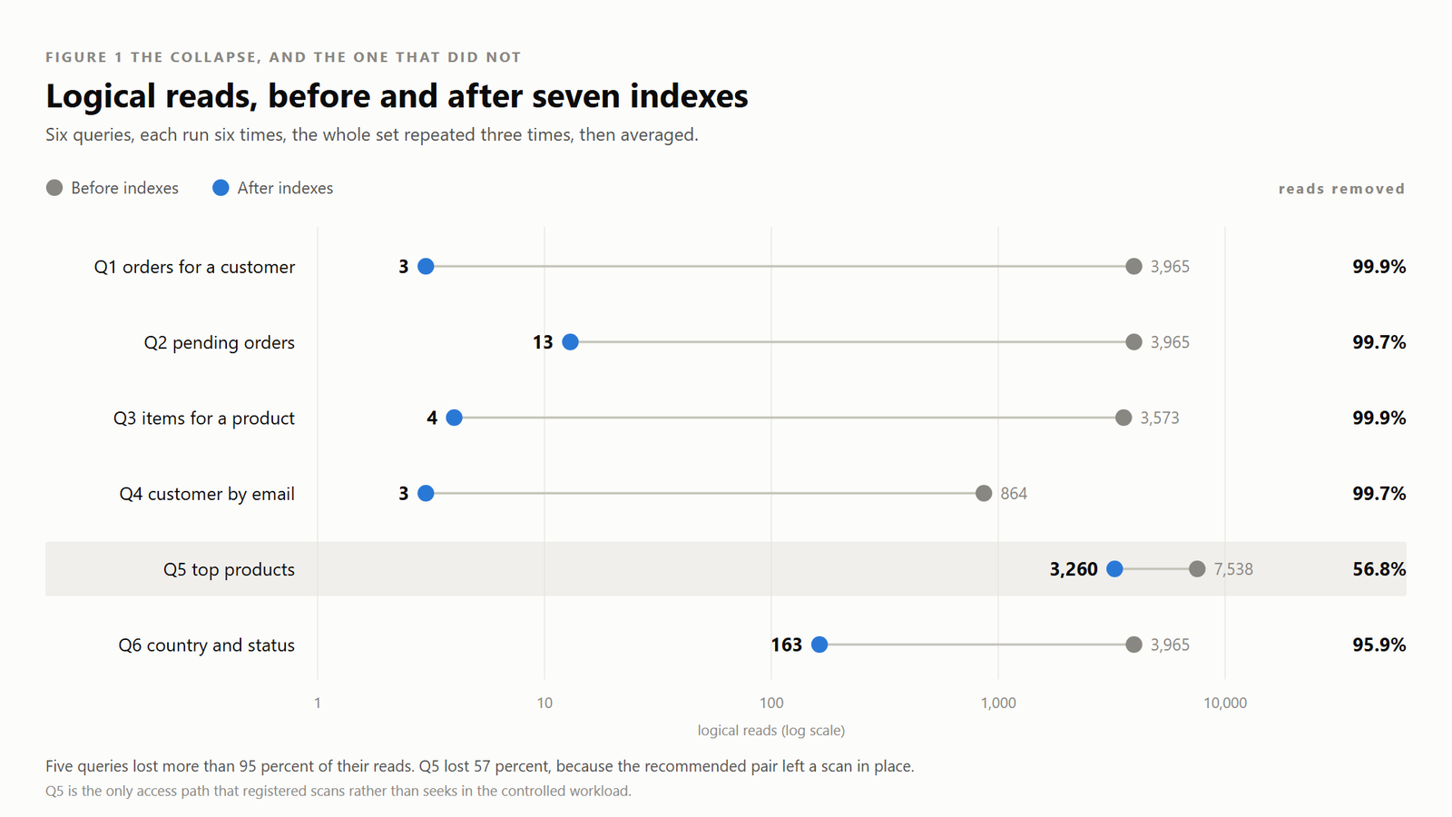
All six queries, on a log scale because three pages and 7,538 pages will not share a linear axis. Five collapsed. One did not.
That makes four indexes from Tuesday, two from Wednesday and one from Q6. Seven in total, and that is the set Thursday’s write test ran against.
Thursday. Then I Looked at the Bill
Sixth query in, seven indexes down, everything faster. So I went looking for what I had not asked the chat model to price.
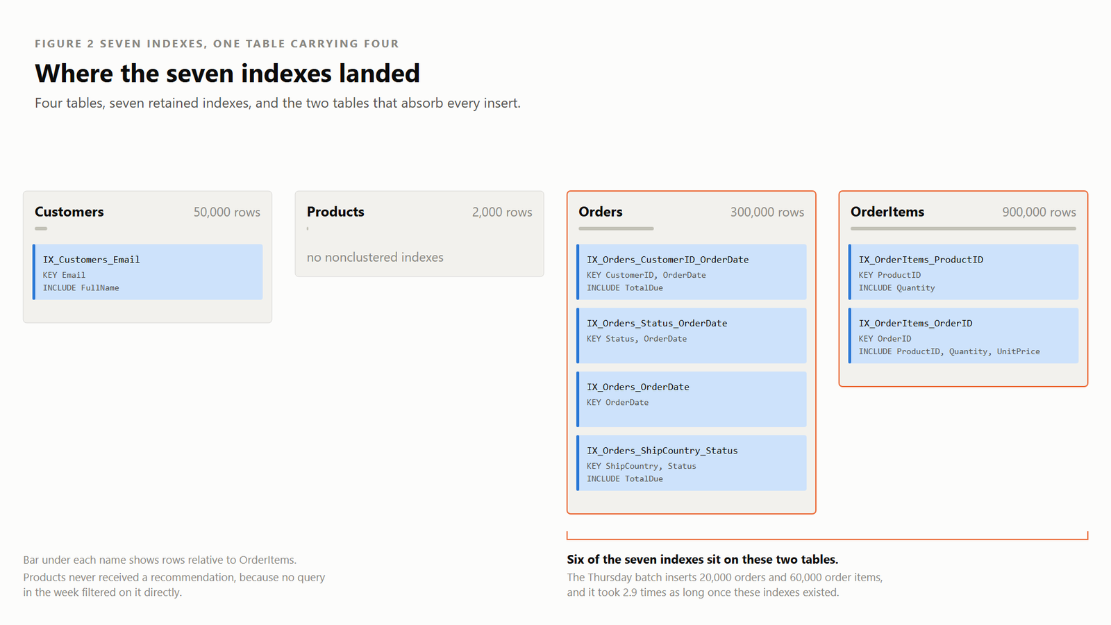
Where the seven landed. Six of them sit on the two tables the insert batch writes to, which is the whole of what follows.
I inserted 20,000 orders and 60,000 order items as one batch, took the median of three runs, and deleted the rows in between. That restores the row count but not the exact physical state, so read this as a strong signal rather than a laboratory benchmark.
| Combined insert batch | No nonclustered indexes | With seven retained indexes |
|---|---|---|
| 20,000 orders and 60,000 order items | 592 ms | 1,703 ms |
This insert batch took 2.9 times as long. My benchmark notes also recorded the space occupied by the four lab tables and their indexes rising from 66 MB to 170 MB. I did not preserve the exact collection query, so that storage figure is context rather than a reproducible measurement.
Not one of those costs appeared in any recommendation. Every answer was about the query in front of it, because the query and the schema were the only evidence I gave it. Ask a model about write cost and it will describe the categories correctly. It cannot price mine without seeing my workload.
Friday. The One I Nearly Misread
A week means new queries arrive. So on Friday I did what everybody does. New slow query, paste it in, ask what index it needs.
SELECT OrderID, Status FROM dbo.Orders WHERE CustomerID = 24680;
-- IX_Orders_CustomerID (CustomerID) INCLUDE (Status)
That is a sensible candidate, and it overlaps an index I already had.
| Index | Key columns | Included columns | Size |
|---|---|---|---|
| IX_Orders_CustomerID | CustomerID | Status | 7 MB |
| IX_Orders_CustomerID_OrderDate | CustomerID, OrderDate | TotalDue | 16 MB |
At first I called the new one redundant because CustomerID is the leftmost key of Tuesday’s index. That would have been a lovely ending and a wrong one. Friday’s query also returns Status, and Tuesday’s index does not contain it. OrderID is available implicitly through the clustered key, but Status is not.
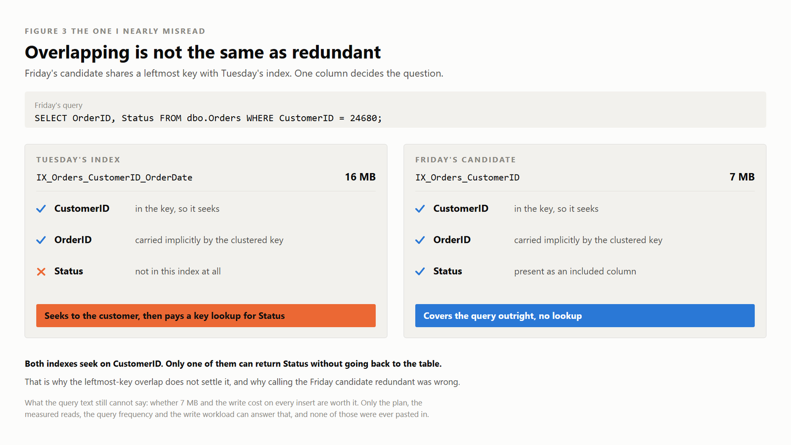
Both seek on CustomerID. Only one of them can return Status without going back to the table.
The Tuesday index can seek to the customer and then look up Status. The Friday candidate can cover the query. It is overlapping, not automatically redundant. A narrower covering index might help a frequent query, or it might add seven megabytes and write work for a benefit too small to matter. Only the actual plan, measured reads, query frequency, and write workload can settle that.
This is still a context failure. Nobody showed the model the index list or the workload. It could propose a locally sensible index, but it could not compare that candidate with the rest of the portfolio. It answered the question it was asked, in a room with no windows. My first interpretation made the same mistake.
The Week, In One Line
Across the first six queries and the seven retained indexes, the week took logical reads from 23,870 down to 3,446, and total duration from 290.1 ms down to 84.7 ms. The combined insert batch moved from 592 ms to 1,703 ms. My benchmark notes recorded the space figure moving from 66 MB to 170 MB, with the collection-method limitation described above. The Friday candidate is not included in those retained-index totals because this experiment did not establish that it deserved to remain.
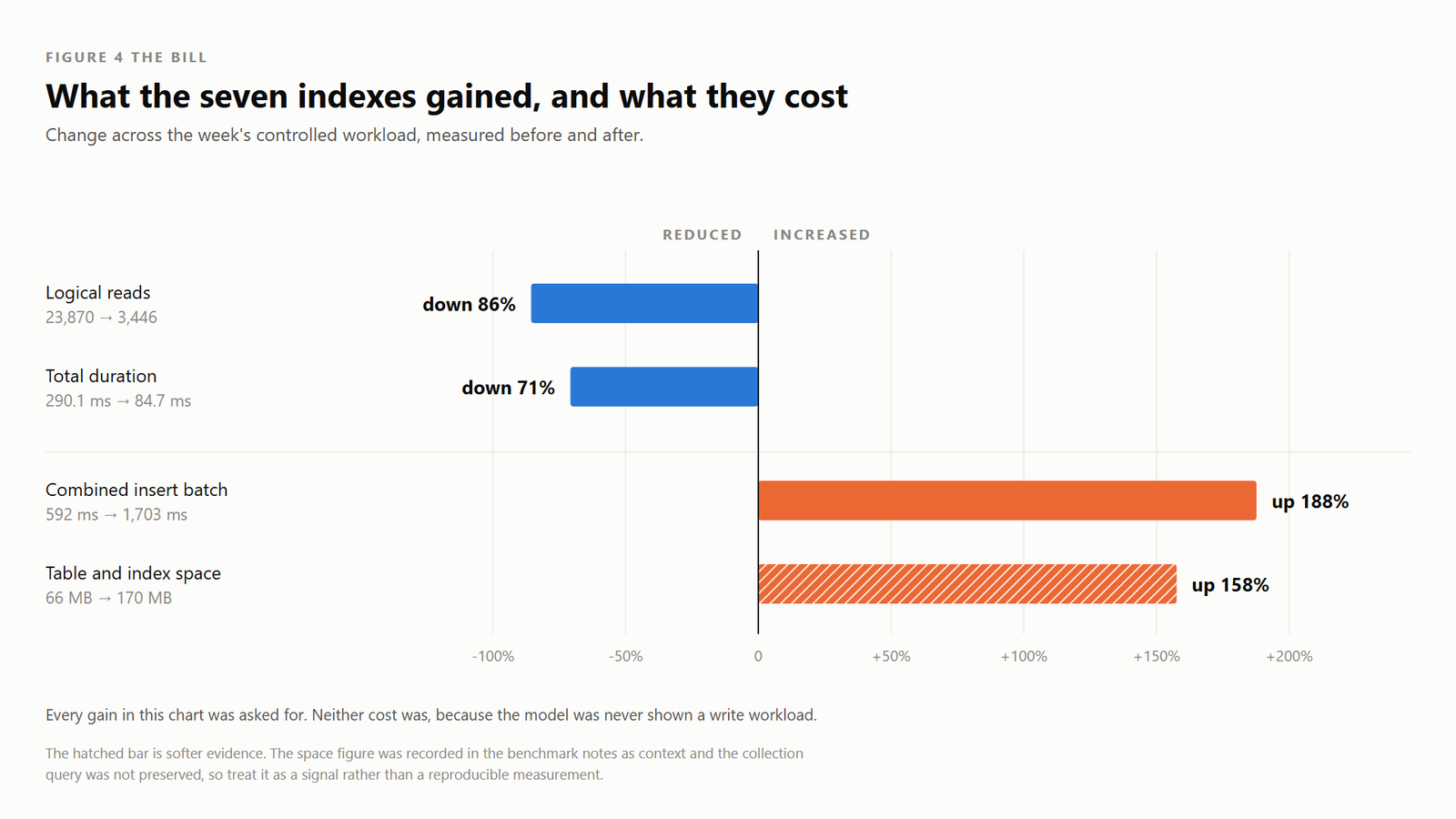
The whole week on one axis. Everything on the left was asked for. Nothing on the right was.
The Good, The Bad and The Ugly
| What happened | The number | |
|---|---|---|
| The Good | The isolated index shapes were useful starting points, and all seven retained indexes registered activity in the controlled workload. That does not prove every one deserves to live forever. | Reads down 86% Duration down 71% |
| The Bad | The stateless recommendations did not price their own advice because I supplied no write workload, storage budget, or maintenance context. | Insert batch took 2.9x as long Recorded space figure 2.6x as large |
| The Ugly | Friday produced an overlapping candidate that could not be judged from the isolated query. My first attempt to call it redundant ignored its included column. | 7 MB candidate Benefit not established |
The ugly one is the part that gets worse over time. Each overlapping index can sound defensible by itself while the portfolio becomes harder to justify.
Would I Do It Again
Yes, and I will. With three changes to how I ask.
Paste the complete existing index definitions in with the query. That means keys and included columns from sys.indexes, sys.index_columns, and sys.columns, not merely the index names. This would have turned Friday into a portfolio discussion instead of another isolated recommendation.
Ask what it might cost, then measure what it actually costs. A model can list likely write, storage, and maintenance effects. It cannot price my workload without workload evidence.
Give it the actual plan, not just the query. Wednesday’s scan would have been visible immediately. That would not guarantee a better index, but it would stop anybody from treating a lower read count as the whole diagnosis.
The pattern I keep landing on this year is always the same. Ask AI a narrow question and you can get a useful narrow answer. The danger is treating that answer as a system-wide decision. A database is a collection of tradeoffs, and a stateless chat sees only the evidence you paste into it.
A stateless answer can be correct about one query and still know nothing about the workload surrounding it.
If you want the wider argument about where this technology genuinely helps and where it quietly does not, that is the subject of all thirty essays in my book AI: Nobody’s in There. But we’re still in here. Every essay is free to read in the complete online collection, and there is a paperback on Amazon if you would rather hold something real.
Run the Smaller Write Test
This smaller lab demonstrates the write cost of one candidate index on the Orders table. It does not reproduce the 2.9x result above because it omits OrderItems and six of the seven retained indexes. Everything lives in temporary tables, so the test leaves nothing behind when the session ends.
Build the 300,000-row temporary table first. Then run the timed block six times without the candidate index, discard the first run, and take the median of the other five.
DROP TABLE IF EXISTS #Orders;
DROP TABLE IF EXISTS #Numbers;

CREATE TABLE #Orders (
    OrderID     int NOT NULL IDENTITY(1,1) PRIMARY KEY CLUSTERED,
    CustomerID  int NOT NULL,
    OrderDate   datetime2(0) NOT NULL,
    Status      varchar(12) NOT NULL,
    TotalDue    decimal(12,2) NOT NULL,
    ShipCountry char(2) NOT NULL,
    Filler      char(60) NOT NULL DEFAULT ''
);

WITH n(x) AS (SELECT 1 UNION ALL SELECT 1 UNION ALL SELECT 1 UNION ALL SELECT 1 UNION ALL
              SELECT 1 UNION ALL SELECT 1 UNION ALL SELECT 1 UNION ALL SELECT 1 UNION ALL
              SELECT 1 UNION ALL SELECT 1),
     t(x) AS (SELECT 1 FROM n a, n b, n c, n d, n e, n f)
SELECT TOP (300000) ROW_NUMBER() OVER (ORDER BY (SELECT NULL)) AS rn
INTO #Numbers FROM t;

INSERT #Orders (CustomerID, OrderDate, Status, TotalDue, ShipCountry)
SELECT 1 + (rn * 7919) % 50000,
       DATEADD(minute, -((rn * 37) % 1051200), '2026-08-01T00:00:00'),
       CASE WHEN rn % 10 < 7 THEN 'Shipped'
            WHEN rn % 10 < 9 THEN 'Pending'
            ELSE 'Cancelled' END,
       CAST(10 + (rn % 90000) / 100.0 AS decimal(12,2)),
       CHOOSE(1 + rn % 6, 'US','GB','IN','DE','AU','CA')
FROM #Numbers;

DROP TABLE #Numbers;
Here is the timed block. The transaction restores the row count even if the test is repeated. The identity value still advances, which is harmless for this temporary lab table and is one more reason not to describe the database as physically identical afterwards.
SET NOCOUNT ON;
SET XACT_ABORT ON;

BEGIN TRANSACTION;

DECLARE @t0 datetime2(7) = SYSDATETIME();

;WITH NewRows AS
(
    SELECT TOP (20000)
           ROW_NUMBER() OVER (ORDER BY (SELECT NULL)) AS rn
    FROM sys.all_objects a
    CROSS JOIN sys.all_objects b
)
INSERT #Orders (CustomerID, OrderDate, Status, TotalDue, ShipCountry)
SELECT 1 + (rn * 7919) % 50000,
       '2026-08-01', 'Shipped', 99.00, 'IN'
FROM NewRows;

SELECT DATEDIFF(millisecond, @t0, SYSDATETIME()) AS InsertMs;

ROLLBACK TRANSACTION;
Now create the candidate index below and run the same timed block six more times. Again, discard the first run and take the median of the other five.
CREATE NONCLUSTERED INDEX IX_Test_Orders_CustomerID_OrderDate
    ON #Orders (CustomerID, OrderDate) INCLUDE (TotalDue);
As a final sanity check, rebuild the temporary table and repeat the comparison in reverse order. Create the index, take the indexed measurements first, run DROP INDEX IX_Test_Orders_CustomerID_OrderDate ON #Orders;, and then take the baseline measurements. This helps expose caching and run-order effects. The comparison answers one narrow question: how much write cost did this one index add to Orders? It does not validate the seven-index, two-table multiplier reported above.
I have run a lot of index reviews over the years, and the ones that go wrong almost never go wrong because somebody chose a bad column. They go wrong because thirty good decisions were made one at a time, by people who could each only see one query.
That is a very old problem. It has just found a very fast new way to happen.
This is not a story about whether AI can suggest an index, it is a story about why a stateless recommendation cannot price a database-wide decision.
Published by Pinal Dave on SQLAuthority. More of my work at pinaldave.com.
Discover more from SQL Authority with Pinal Dave
Subscribe to get the latest posts sent to your email.